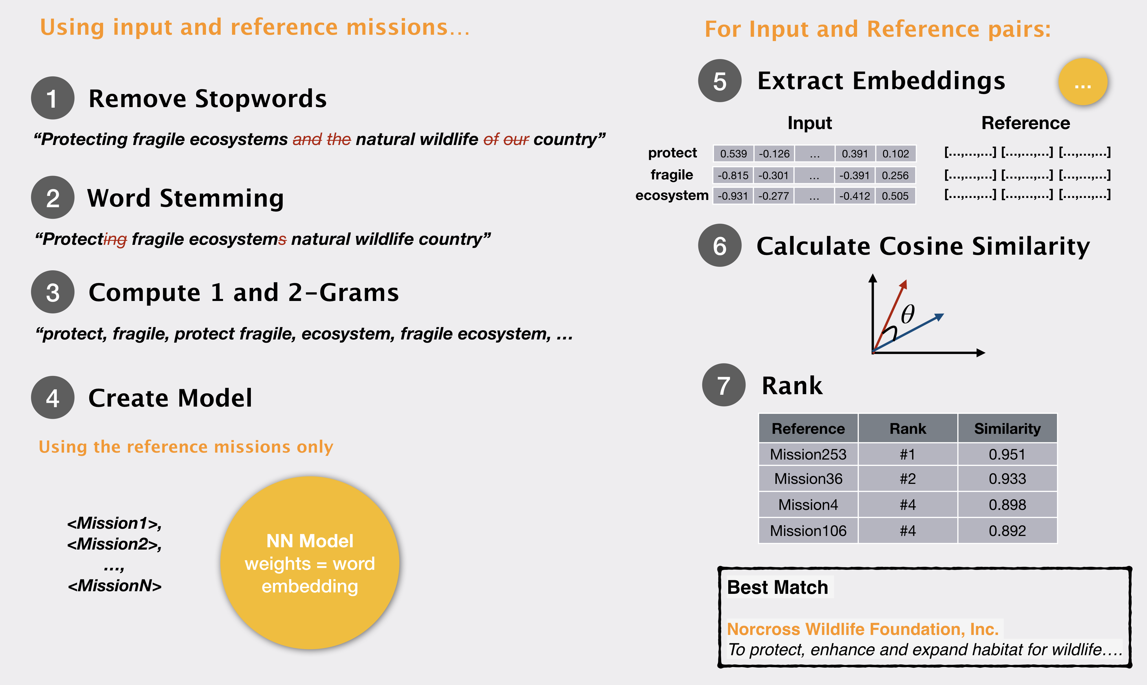
In our previous post, we noted how 1 and 2 grams from a query mission can be matched to donor mission statements to find an appropriate donor organization. We performed some text cleaning and used
What if, instead of computing simple word matching statistics, we could encode a lot more information about the word – rather than a few numerical values that we compute, we store each word as some n-dimensional vector, encoding various properties of its meaning, and usage?Word embeddings are a way of representing a word along with the meaning/context it is found in. In this representation a word becomes a vector – or a series of numbers – that signify the word meaning. Now if one word vector ‘matches’ another word vector we can say that the two words match in meaning and context.
In this
# Loading Libraries
library(tidyverse)
library(tidytext)
library(wordVectors)
library(SnowballC)
# read the reference missions
guidestar <- read_csv("data/guidestar_full.csv")

# tokenizing and removing stopwords
guidestar_words <- guidestar %>%
    mutate(Mission = paste(Organization, Mission)) %>%
    unnest_tokens(word, Mission, drop = FALSE) %>%
    anti_join(stop_words) %>%
    mutate(word = wordStem(word, language = "english"))
# get in text format for training
guidestar_clean <- guidestar_words %>%
    select(EIN, Organization, word) %>%
    group_by(Organization) %>%
    summarise(Mission = paste(unique(word), collapse = " "))

full_text <- tolower(paste(guidestar_clean$Mission, collapse = "\n"))

writeLines(full_text, "training_temp.txt")

tmp_file_txt <- "training_temp.txt"
We create the model with the default params. The model here does a prediction for finding the probability that a word appears along with other words in the text. The weights that the model learns in this process become our word representation (or word embedding). To view the results and see whether the model has
# prep the doc
prep_word2vec("training_temp.txt", destination = "training_complete.txt",
              lowercase = TRUE, bundle_ngrams = 2)
word2vec_model1 <- train_word2vec("training_complete.txt", "word2vec_vectors1.bin",
                                vectors = 200, min_count = 2, threads = 4,
                                 window = 12, iter = 5,
                                 negative_samples = 0,
                                 force = TRUE)

close_words <- closest_to(word2vec_model1,
                        word2vec_model1[[c("diabet")]],
                        n = 10)
close_words_vec <- word2vec_model1[[close_words$word, average=F]]
plot(close_words_vec, method="pca")
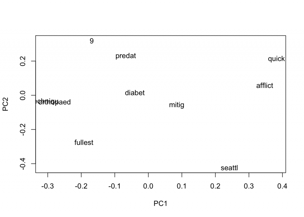
In the
Let us also try to reduce the window size and see how that affects. A smaller window would tend to give us more related words, in theory.
word2vec_model2 <- train_word2vec("training_complete.txt", "word2vec_vectors2.bin",
                                 vectors = 30, threads = 4,
                                 window = 7, min_count = 2,
                                 negative_samples = 4, iter = 10,
                                 force = TRUE)
close_words <- closest_to(word2vec_model2,
                        word2vec_model2[[c("diabet")]],
                        n = 10)
close_words_vec <- word2vec_model2[[close_words$word, average=F]]
plot(close_words_vec, method="pca")
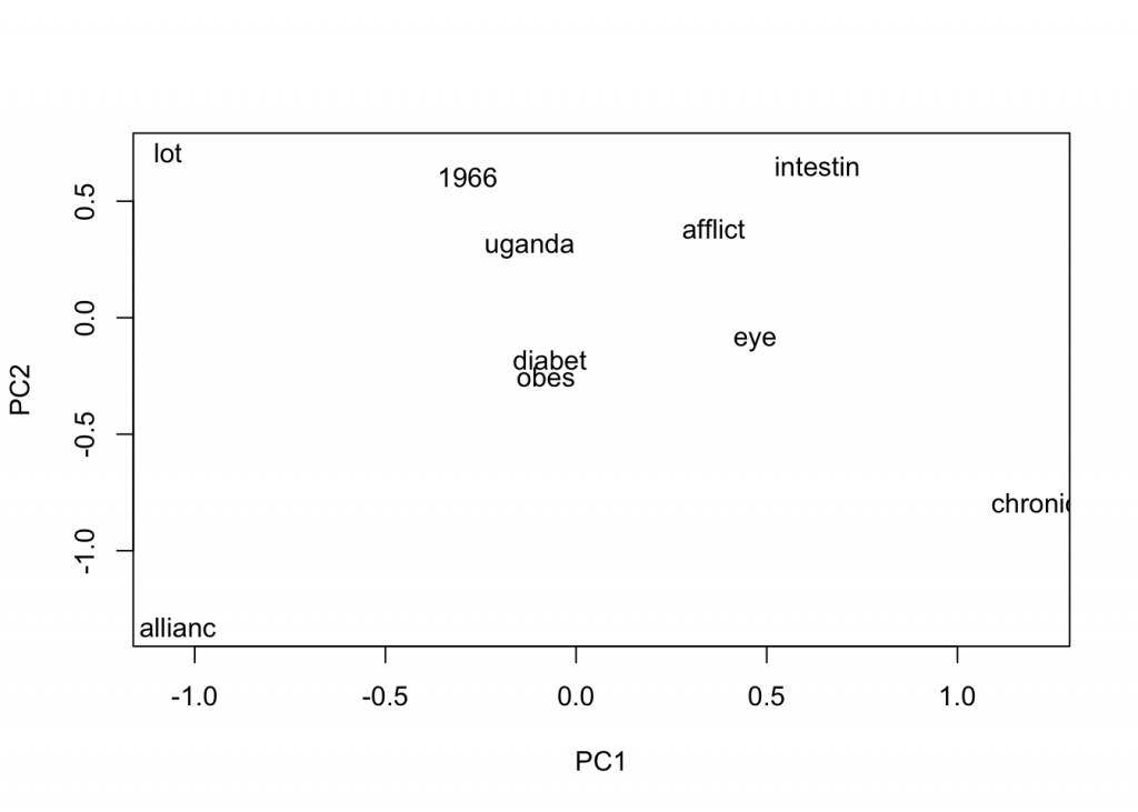
These words look much better! We see “obes” for obesity, “afflict”, and “eye”. So let’s choose model 2 and build the word representation for words in the query mission.
query <- "We aim to promote awareness of serious heart conditions and work to provide treatment for those with heart disease, high blood pressure, diabetes, and other cardiovascular-related diseases who are unable to afford it"

query_words <- query %>%
    as.data.frame %>%
    select(Query = 1) %>%
    mutate(Query = tolower(as.character(Query))) %>%
    unnest_tokens(word, Query) %>%
    anti_join(stop_words) %>%
    mutate(word = wordStem(word, language = "english"))

# vector representations for the query and references
mat1 <- word2vec_model2[[unique(query_words$word), average = FALSE]]
mat2 <- word2vec_model2[[guidestar_words$word, average = FALSE]]

similarities <- cosineSimilarity(mat1, mat2)

# taking an approx measure of the similarity
highest_matching_words <- colSums(similarities)

matching_df <- data.frame(word = names(highest_matching_words), sim = as.numeric(highest_matching_words), stringsAsFactors = FALSE)

# viewing results
res <- guidestar_words %>%
    select(EIN, Mission, word) %>%
    left_join(matching_df) %>%
    group_by(EIN, word) %>%
    group_by(EIN) %>%
    summarise(Mission = Mission[!is.na(Mission)][1],
              Score = mean(sim, na.rm = TRUE)) %>%
    arrange(desc(Score))

res %>%
    slice(1:5) %>%
    knitr::kable()
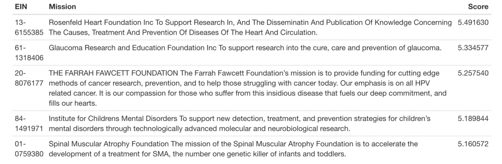
Our results are much better! We see that “Israel at heart” is not a match
Leave a Reply
You must be logged in to post a comment.